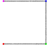
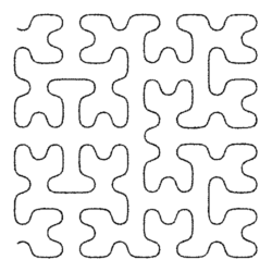
Hilbert Curve
Concepts & Implementation


return to main index


Introduction

The web notes by Andrew Cumming of Napier University Edinburgh provide a very good introduction to the Hilbert curve. His pseudo code, slightly modified, is shown in listing 1.


Listing 1 (from Andrew Cumming)


procedure hilbert(x, y, xi, xj, yi, yj, n)
/* x and y are the coordinates of the bottom left corner */
/* xi & xj are the i & j components of the unit x vector of the frame */
/* similarly yi and yj */
if (n <= 0) then
   LineTo(x + (xi + yi)/2, y + (xj + yj)/2);
else
   {
   hilbert(x,           y,           yi/2, yj/2,  xi/2,  xj/2, n-1);
   hilbert(x+xi/2,      y+xj/2 ,     xi/2, xj/2,  yi/2,  yj/2, n-1);
   hilbert(x+xi/2+yi/2, y+xj/2+yj/2, xi/2, xj/2,  yi/2,  yj/2, n-1);
   hilbert(x+xi/2+yi,   y+xj/2+yj,  -yi/2,-yj/2, -xi/2, -xj/2, n-1);
   }
end procedure;

To fully understand how Andrews recursive function operates is not easy and in order to do so it is necessary to break-down his Hilbert procedure so that the role that each "part" plays in the construction of the curve can be more readily understood. We will begin by looking at the inputs of the Hilbert function.


Inputs

In addition to the counter (n) that tracks the level from which the function begins to recursively call itself, there are six other inputs to Andrew's procedure. The first two define the x and y coordinates of an input point that will be used in the calculation of a point on the Hilbert curve. The next 4 values define two vectors. Before we see how they are used we must understand what is meant by the inputs labelled xi, xj, yi and yj. Hopefully, figure 1 will make them clearer.

The large black dot, labelled P, in figure 1 is defined by its x and y coordinates - shown as small dots on the two axes. We can see, from the two arrows, that each dot marks the head of a vector. We might call these the x-vector and the y-vector.


Figure 1


Although these vectors represent the x and y coordinates of P, like any vector, they have their own coordinates. For example, the coordinates of the x-vector (in two dimensions) might be [1,0] while the coordinates of the y-vector might be [0,0.5]. To prevent the confusion of labelling the coordinates of these vectors as "x" and "y" they are instead labelled "i" and "j". For example,

    x-vector              y-vector
    xi = 1.0              yi = 0.0 
    xj = 0.0              yj = 0.5

We can make use of these vectors to move (ie. translate) a copy of point P. For example, in Andrew's procedure we see this statement.

    LineTo(x + (xi + yi)/2, y + (xj + yj)/2);

Rewritten for point P we have,

    Px = Px + (xi + yi)/2
       = 1.0 + (1.0 + 0)/2
       = 1.5

    Py = Py + (xj + yj)/2
       = 0.5 + (0 + 0.5)/2
       = 0.75

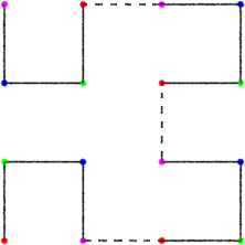
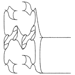
The effect of using the i's and j's on point P can be seen in figure 2.


Figure 2


Point P could also have been translated by directly changing its x and y values. However, using the "i" and "j" coordinates (x-vector and y-vectors) moves the point in a structured and proportional fashion. In the context of their use in Andrew's procedure, the "i" and "j" components provide, what are in effect, additional "handles" to control the placement of points along the Hilbert curve.


Modifying the Inputs

Looking at the hilited code shown in listing 2 we see the Hilbert procedure calls itself four times. On each call it passes slightly modified versions of its original input values to itself.


Listing 2 (pseudo code)


procedure hilbert(x, y, xi, xj, yi, yj, n)
if (n <= 0) then
   LineTo(x + (xi + yi)/2, y + (xj + yj)/2);
else
   {
   hilbert(x,           y,           yi/2, yj/2,  xi/2,  xj/2, n-1);
   hilbert(x+xi/2,      y+xj/2 ,     xi/2, xj/2,  yi/2,  yj/2, n-1);
   hilbert(x+xi/2+yi/2, y+xj/2+yj/2, xi/2, xj/2,  yi/2,  yj/2, n-1);
   hilbert(x+xi/2+yi,   y+xj/2+yj,  -yi/2,-yj/2, -xi/2, -xj/2, n-1);

   }
end procedure;

    //      x  y  xi  xj  yi  yj  n
    hilbert(0, 0, 1,  0,  0,  1,  1);

Tracking the results of the recursions will show what happens to original x,y coordinates - shown in above in blue. The i and the j vectors will be ignored. The four recursive calls will be labelled A, B, C and D ie.

    A    hilbert(...);
    B    hilbert(...);
    C    hilbert(...);
    D    hilbert(...);

Performing the arithmetic on the x and y's for the first level of recursion for A, B, C and D generates the following x,y values,

                  x    y
    A    hilbert(0.0  0.0, ...);
    B    hilbert(0.5  0.0, ...);
    C    hilbert(0.5  0.5, ...);
    D    hilbert(0.5  1.0, ...);

The value of x and y can be plotted using the LineTo - listing 3.


Listing 3 (pseudo code)


procedure hilbert(x, y, xi, xj, yi, yj, n)
if (n <= 0) then
   LineTo(x  + (xi + yi)/2, y  + (xj + yj)/2");
else
   {
   hilbert(x,           y,           yi/2, yj/2,  xi/2,  xj/2, n-1);
   hilbert(x+xi/2,      y+xj/2 ,     xi/2, xj/2,  yi/2,  yj/2, n-1);
   hilbert(x+xi/2+yi/2, y+xj/2+yj/2, xi/2, xj/2,  yi/2,  yj/2, n-1);
   hilbert(x+xi/2+yi,   y+xj/2+yj,  -yi/2,-yj/2, -xi/2, -xj/2, n-1);
   }
end procedure;

Figures 3 to 6 show the development of a Hilbert curve from 1 to 4 iterations. The colored dots correspond to the four recursions ie.

    A    hilbert(...); red dot
    B    hilbert(...); green dot
    C    hilbert(...); blue dot
    D    hilbert(...); purple dot

Figure 3 shows the basic building block of the Hilbert curve is a open square formed by three connected lines. A complex pattern (figure 4) is made by the Hilbert procedure recursively converting each line to a smaller version of the original open square. The lines of each of the small squares are then converted to even smaller squares, and so on, and so on. After one iteration we have four smaller separate squares. Because of the way the vertices of each square are drawn the final pattern is formed by a single continuous line. In figure 4 the connections that join the small (separate) open squares are shown as dotted lines.


Figure 3
Starting Open Square


Figure 4
Afer one Interation


Figure 5
3 interations


Figure 6
4 interations


Basic Code

Listings 4 and 5 provide code for a RenderMan procedural primitive. One is written in Python, the other in Tcl. For information about procedural primitives, or helper apps as they are often called, refer to the tutorial,
    RenderMan Procedural Primitives: Implementations in Python, Tcl and 'C'
A sample rib file to run the implementations is given by listing 6.


Listing 4 (hilbert.py)


import sys, math
  
def hilbert(x0, y0, xi, xj, yi, yj, n):
    if n <= 0:
        X = x0 + (xi + yi)/2
        Y = y0 + (xj + yj)/2
        
        # Output the coordinates of the cv
        print '%s %s 0' % (X, Y)
    else:
        hilbert(x0,               y0,               yi/2, yj/2, xi/2, xj/2, n - 1)
        hilbert(x0 + xi/2,        y0 + xj/2,        xi/2, xj/2, yi/2, yj/2, n - 1)
        hilbert(x0 + xi/2 + yi/2, y0 + xj/2 + yj/2, xi/2, xj/2, yi/2, yj/2, n - 1)
        hilbert(x0 + xi/2 + yi,   y0 + xj/2 + yj,  -yi/2,-yj/2,-xi/2,-xj/2, n - 1)
        
def main():
    args = sys.stdin.readline()
    # Remain the loop until the renderer releases the helper...
    while args:
        arg = args.split()
        # Get the inputs
        pixels = float(arg[0])
        ctype = arg[1]
        reps = int(arg[2])
        width = float(arg[3])
        
        # Calculate the number of curve cv's
        cvs = int(math.pow(4, reps))
            
        # Begin the RenderMan curve statement
        print 'Basis \"b-spline\" 1 \"b-spline\" 1'
        print 'Curves \"%s\" [%s] \"nonperiodic\" \"P\" [' % (ctype, cvs)
    
        # Create the curve
        hilbert(0.0, 0.0, 1.0, 0.0, 0.0, 1.0, reps)
    
        # End the curve statement
        print '] \"constantwidth\" [%s]' % width
      
        # Tell the renderer we have finished   
        sys.stdout.write('\377')
        sys.stdout.flush()
        
        # read the next set of inputs
        args = sys.stdin.readline()
if __name__ == "__main__":
    main()


Listing 5 (hilbert.tcl)


fconfigure stdout -translation binary
  
# This is where the control vertices of the Hilbert curve are generated    
proc hilbert { x0 y0 xi xj yi yj n } {
    if { $n <= 0 } {
        set X [expr $x0 + ($xi + $yi)/2]
        set Y [expr $y0 + ($xj + $yj)/2]
        
        # Output the coordinates of the cv
        puts "$X $Y 0 "
    } else {
        set XI [expr $xi/2]
        set XJ [expr $xj/2]
        set YI [expr $yi/2]
        set YJ [expr $yj/2]
        
        # Begin recursion
        hilbert $x0                 $y0                $YI  $YJ  $XI  $XJ [expr $n - 1]
        hilbert [expr $x0+$XI]     [expr $y0+$XJ]      $XI  $XJ  $YI  $YJ [expr $n - 1]
        hilbert [expr $x0+$XI+$YI] [expr $y0+$XJ+$YJ]  $XI  $XJ  $YI  $YJ [expr $n - 1]
        hilbert [expr $x0+$XI+$yi] [expr $y0+$XJ+$yj] -$YI -$YJ -$XI -$XJ [expr $n - 1]
        }
    }
  
# Remain the loop until the renderer releases the helper...
while { [gets stdin args] != -1 } {
    # Get the inputs
    set pixels [lindex $args 0]
    set ctype  [lindex $args 1]
    set reps   [lindex $args 2]
    set width  [lindex $args 3]
  
    # Calculate the number of curve cv's
    set cvs [expr int(pow(4, $reps))]
        
    # Begin the RenderMan curve statement
    puts "Basis \"b-spline\" 1 \"b-spline\" 1"
    puts "Curves \"$ctype\" \[$cvs\] \"nonperiodic\" \"P\" \["
    
    # Create the curve
    hilbert 0.0  0.0  1.0  0  0  1.0 $reps
    
    # End the curve statement
    puts "\] \"constantwidth\" \[ $width \]"
  
    # Tell the renderer we have finished   
    puts "\377" 
    flush stdout
    }

The inputs (arguments) to the helper apps are,
    curve type - either linear or cubic
    number of iterations
    width of the curve


Figure 7
cubic - 4 iterations


Listing 6 (hilbert.rib)


Display "iterations" "framebuffer" "rgba"
Format 300 300 1
Projection "perspective" "fov" 12
ShadingRate 1
  
Translate  -0.5 -0.5 5
Rotate 0 1 0 0
Rotate 0   0 1 0
Scale 1 1 -1
WorldBegin
    TransformBegin
        Surface "constant"
        Color 1 1 1
        # For linux and MacOSC the paths to tclsh and
        # python must be fully specified ie,
        # /usr/bin/tclsh
        # /usr/bin/python
        # Args: curve type, iterations and curve width
        Procedural "RunProgram" ["tclsh  FULL_PATH/hilbert_helper.tcl" "cubic 4 0.005"] 
                    [-1 1 -1 1 -1 1]
        #Procedural "RunProgram" ["python  FULL_PATH/hilbert_helper.py" "linear 4 0.005"] 
        #           [-1 1 -1 1 -1 1]
    TransformEnd
WorldEnd


Mistakes can be Interesting

When entering the code for the Python and Tcl scripts I made a couple of mistakes that produced some interesting results. The first error occured in a python script.

hilbert(x0,               y0,               yi/2, yj/2, xi/2, xj/2, n - 1)
hilbert(x0 + xi/2,        y0 + xj/2,        xi/2, xj/2, yi/2, xj/2, n - 1)
hilbert(x0 + xi/2 + yi/2, y0 + xj/2 + yj/2, xi/2, xj/2, yi/2, xj/2, n - 1)
hilbert(x0 + xi/2 + yi,   y0 + xj/2 + yj,  -yi/2,-yj/2,-xi/2,-xj/2, n - 1)


Figure 8


The second error occured a tcl script.

hilbert $x0                    $y0                     $YI  $YJ  $XI  $XJ [expr $n - 1]
hilbert [expr $x0 + $XI]       [expr $y0 + $XJ]        $XI  $XJ  $YI  $YJ [expr $n - 1]
hilbert [expr $x0 + $XI + $YI] [expr $y0 + $XJ + $YJ]  $XI  $XJ  $YI  $YJ [expr $n - 1]
hilbert [expr $x0 + $XI + $YI] [expr $y0 + $XJ + $yj] -$YI -$YJ -$XI -$XJ [expr $n - 1]


Figure 9


© 2002- Malcolm Kesson. All rights reserved.